Once you head away from the areas that are serviced by modern terrestrial cable infrastructure, the available digital communications options are somewhat limited. Some remote areas are served using High Frequency radio systems, using radio signals that bounce off the ionosphere to provide a long distance, but limited bandwidth, service. Or there are satellite-based services, based on spacecraft positioned in geostationary orbital slots.
These geostationary satellite systems can offer far greater bandwidth than high frequency radio but have significantly higher latency as the satellite is orbiting at 35,786 km above the equator in order to synchronise the orbital period with the earth’s revolution. For a signal to travel to the spacecraft and back, will take a minimum of 239ms of signal propagation time (assuming that the earth end is directly under the spacecraft on the equator).
In the context of Internet communications, a satellite hop will add at least 477ms to a round trip time (RTT) measurement, as a signal will need to head up to the satellite and back twice for the complete round trip. When the earth end points move away from directly under the spacecraft, then these paths will be longer. At the horizon of satellite visibility, the distance to the spacecraft is 42,640km away, and the signal propagation time is 284ms, or 568ms as a RTT value (Figure 1).

Figure 1 – the Geometry of Geo-Stationary Satellites
When you add switching delays and terrestrial components, and use a land point in the mid-latitudes, a circuit that includes a satellite hop will generally see RTT measurements of around 600ms. Network queues will add to this delay, of course.
Into this mix we are now seeing the introduction of Low Earth Orbit (LEO) services, which can offer the potent combination of higher bandwidth and lower latency. Low Earth Orbits start at altitudes low as 160km and as high as 2,000km. The objective is to keep the satellite’s orbit high enough to stop it slowing down by “grazing” the denser parts of the earth’s ionosphere, but not so high that it loses the radiation protection afforded by the Inner Van Allen belt. At a height of 550km, the minimum signal propagation delay to reach the satellite and back is 3.7ms.
There are a number of LEO systems being announced, launched and bought into service. As well as SpaceX’s Starlink’s service, there is also OneWeb, with some 428 satellites in its constellation and a further 220 or so satellites planned for launch. OneWeb uses a higher orbital plane, at an altitude of 1,200 km, and the satellites use a polar orbit, compared to Starlink’s inclined orbits. Amazon’s FCC filings for its proposed Kuiper LEO constellation describe a planned constellation of up to 3,300 satellites. Boeing has obtained regulatory permission to launch some 150 LEO broadband spacecraft. There is also a Chinese project underway.
Communicating with LEO satellites is quite different to GEO satellites. LEO satellites move quickly across the sky, but are relatively close to the earth, so there is no need to use a large heavy steerable dish antenna. For LEO systems it is possible to use a phased array panel to direct the focus of the antenna to each satellite as it passes overhead.
The LEO system we will be testing here is Starlink. As of March 2022, a total of 2,335 Starlink spacecraft have been launched, with 2,110 still in orbit. Of those, 1,608 are in the licensed operational shells and 447 are undergoing orbit raising towards those shells.
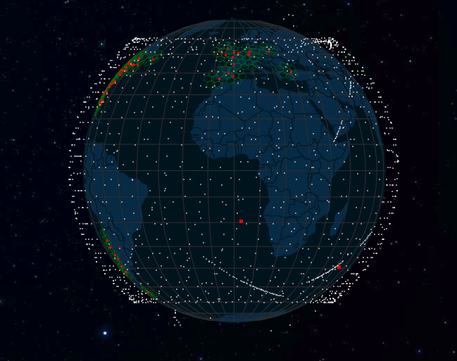
Starlink satellite map – from https://satellitemap.space
The Starlink satellites currently communicate to ground stations, and not to each other, which limits the extent of areas served by Starlink, as each active satellite has to be in range of an earth station in order to provide service.
While these satellites orbit at an altitude of 550km, they appear over the horizon at a distance of 2,705km. The satellites have velocities of around 7.6 km/sec, and have an orbital period of around 95 minutes, so each satellite is visible from horizon to horizon for 12 minutes. This corresponds to a relative change of 1 degree of elevation every 15 seconds. In practice, the range of useful visibility of these satellites is far more restricted than this.
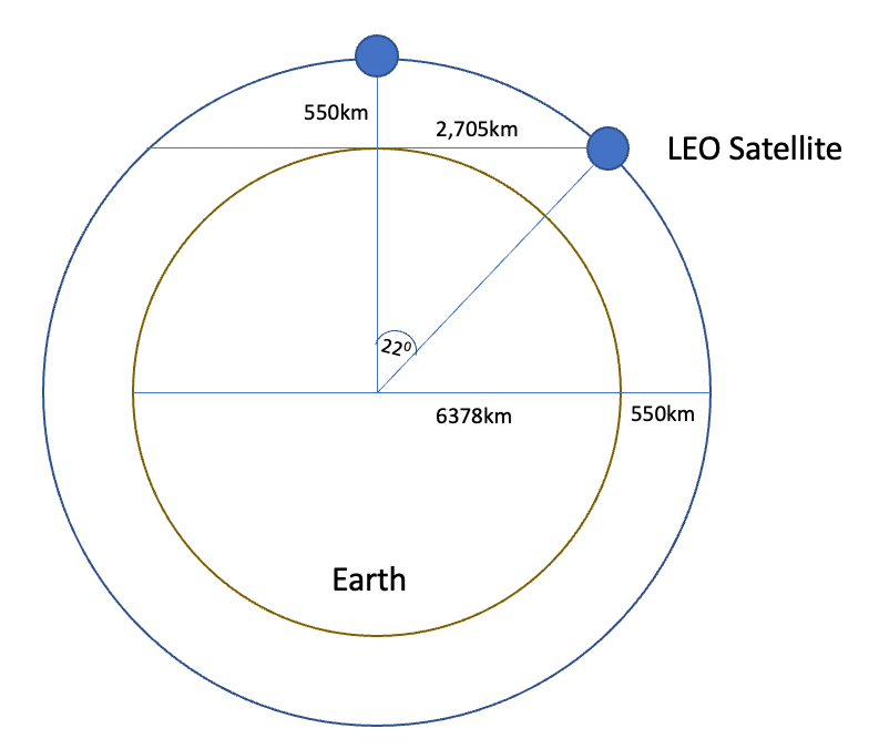
Figure 2 – the Geometry of LEO Satellites
Currently these satellites are “mirrors in the sky” and need to have line of sight to both the end user and an earth station to provide a service. Starlink are planning to use inter-satellite communications with laser links, which will extend its potential coverage to most parts of the Earth. This would also improve the end-to-end signal propagation speed by up to 50% by replacing long distance fibre optic hops with inter-satellite laser signals.
In Australia there is a large amount of rural and remote areas which are not well served by wired services. These days there are two connection options for rural and remote. Firstly, there is a system based on 2 geo-stationary satellites and ten ground stations that offers an Internet access service that is rate managed per user to a maximum of 25Mbps per user. This is the Australian National Broadband Network’s “Sky Muster” service. Secondly, in certain parts of the country there is the Starlink service. Starlink can offer service speeds up to some 90Mbps download and 14Mbps upload.
We’ve been interested in comparing the achieved protocol performance of these two satellite services for some time, and in early 2022 we had to opportunity to place a monitoring unit at a remote site which is connected to both Starlink and Sky Muster services. This is a report of what we found when we tested both services with a number of different TCP protocols.
TCP Congestion Control Protocols
There are three TCP flow control protocols in widespread use today. These are sender-side algorithms that control the amount of data being passed into the network based on the network state that is inferred by the incoming ACK stream. The ideal steady state for all these TCP flow control algorithms is to pass new segments of data into the network at the same rate as the receiver removes segments from the network. If the protocol can discover the available capacity of the network path, then the algorithm will operate efficiently across the network. However, the path capacity of the network is unknown and subject to change because of the interaction with other data flows. The way these protocols adapt to this situation is to increase the sending rate to probe the network with increased sending rates and react by decreasing the sending rate when it receives an indication that its sending rate is greater than the patch capacity. The way these protocols achieve this is by changing the size of the sender’s sending window, or congestion window (cwnd).
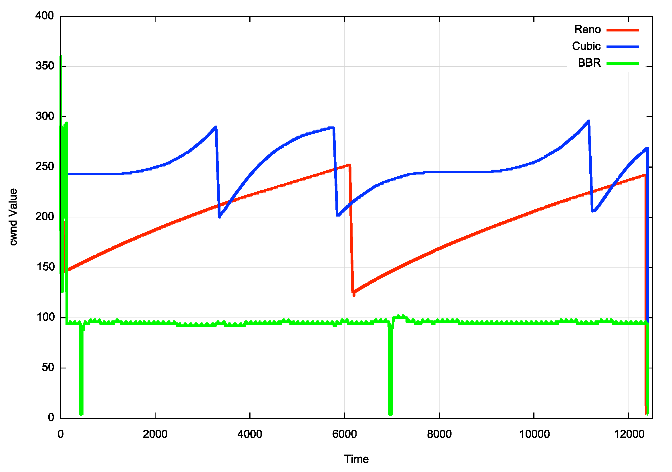
Figure 3 – cwnd management for TCP flow control Protocols
Reno is the currently used version of the conventional Additive Increase Multiplicative Decrease (AIMD) TCP flow control algorithm. This protocol increases cwnd by 1 segment every RTT until it encounters packet loss. Upon receipt of a loss signal (duplicate ACK) it halves the cwnd value and then resumes its linear inflation of cwnd. This algorithm will slowly fill the network queues with data. Assuming that the network operator has dimensioned these queues at a size that is the delay x bandwidth product of the link that is driven by the queue, then when the queues are full and congestion drop happens, the network contains twice the delay x bandwidth product of the end-to-end path. By rate-halving at this point Reno allows the network queues to drain, and at this point it resumes its linear increase of cwnd. This behaviour of cwnd is shown in Figure 3, in the red trace.
Cubic has been adopted by many Linux systems as the congestion control protocol of choice. Cubic attempts to hold the cwnd value at a level which is sustainable by the network for longer intervals. When it probes upward into higher sending rates it does so cautiously at first, then increases rapidly if no loss signal is received. The way it achieves this is by using a cwnd inflation function which is based on a Cubic polynomial function. Cubic reduces the cwnd value by 1/3 when it sees packet drop. This behaviour is shown in Figure 3, in the blue trace.
BBR uses a different approach to flow control. Once it has an estimate of the delay x bandwidth product of the network path it maintains the sending rate at this setting for 6 x RTT intervals. On the 7th interval it increases the sending rate by 25% and on the next it drops the sending rate by the same amount. If BBR’s network capacity estimate is too low then the pulse of increased traffic will be handled by the work without the formation of queues, so the RTT of these packets will remain steady. In this case BBR will increase its estimate of the delay x bandwidth product of the network path. If the pulse of increased traffic causes a rise in the RTT of these packets then this is a signal that network queues are forming, and the sending rate should not be altered. The BBR management of cwnd is shown in Figure 3, in the green trace.
However, these days there are a number of additional factors that also govern TCP performance. TCP Selective Acknowledgement (SACK) allows TCP sessions to recover from lost packets without closing down the TCP windows. TCP Timestamp options allow the TCP systems to have a more accurate view of the routing trip time between the end systems. Explicit Congestion notification (ECN) allows the TCP session to be informed on network congestion before the onset of queue drop. The internal queuing disciplines have become more intricate. These local optimisations allow the TCP session to maintain a more accurate view of the capacity of the network path, and more importantly, allow a TCP sender to maintain a sending rate that does not necessarily push the network into regular queue buildup and congestion loss. In other words, while the internal cwnd TCP control variable behaves as per the flow control model, the packet sending behaviour on modern Linux systems is able perform with a far better level of adaptation to the available path capacity.
What we are primarily interested in here is the ability of these modern TCP implementations to efficiently use the network across network paths that use geostationary and LEO satellite components.
The Control: Terrestrial Fibre
Firstly, as a control point, let’s look at the other end of the spectrum of retail consumer connectivity options in Australia as a control point for the satellite measurements. The service we will use as a reference point is a fibre-based service which delivers 275Mbps/25Mbps.
This measurement uses an on-site Intel NUC device running Debian 10 as the client, and the server is a Dell unit, again running Debian 10. The server is located in Brisbane, Australia and the on-site fibre-tail connected device is in Canberra, Australia, locations that are some 1,000km apart.
For the Fibre test the path between server and the on-site device has a minimum round-trip time (RTT) of 19.5ms with a mean of 1.1ms of additional network queuing delay in IPv4. When using IPv6 the Ping results show a minimum 19.622ms RTT, with a mean of 0.9ms of additional network queuing delay (Figure 4). IPv4 is slightly faster in this test environment, due to a slightly different internal path through the provider’s infrastructure.
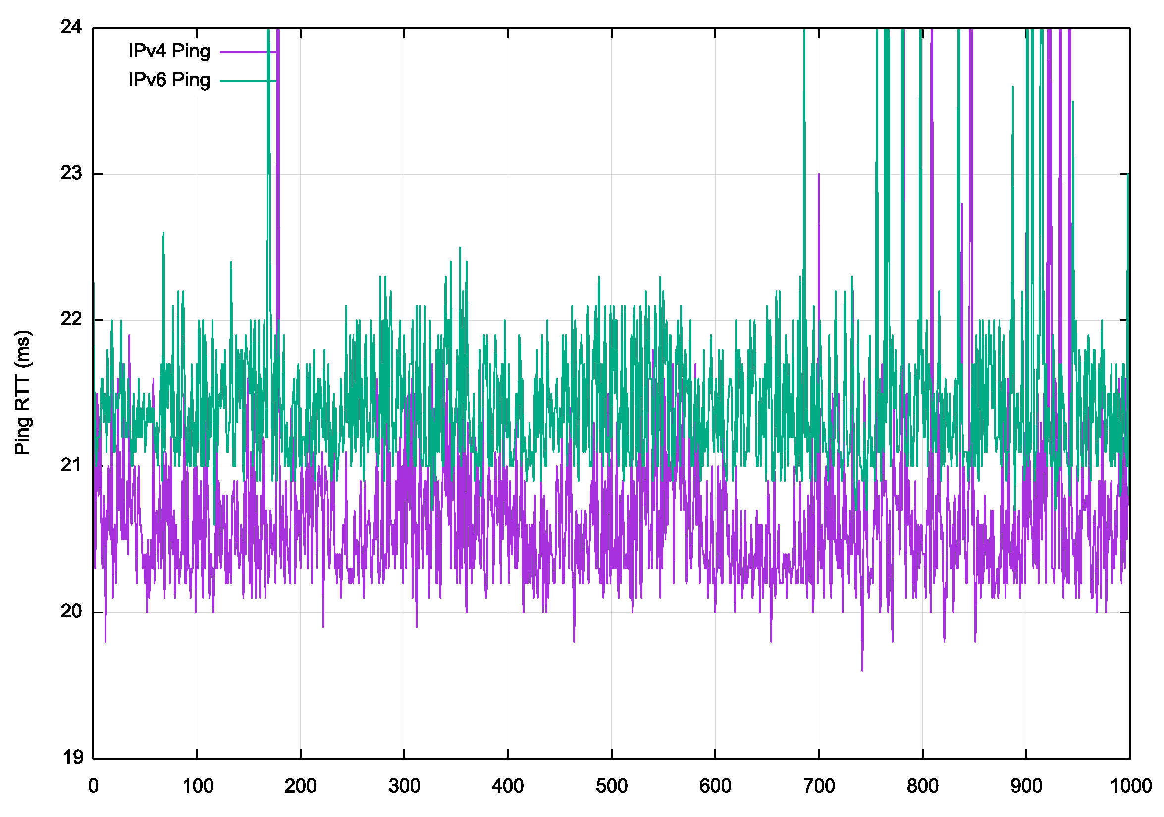
Figure 4 – Ping measurements of the RTT for IPv4 and IPv6
For this measurement we will be running TCP sessions that download a data stream from the server to the client. The measurement will start with a single stream, then 20 seconds later a second stream is added. 100 seconds later the initial stream is terminated, and the second stream continues for a further 20 seconds.
Figure 5 shows the results of this on the downstream fibre link, which is provisioned at a sending rate of 275Mbps, using the Reno TCP flow control protocol.
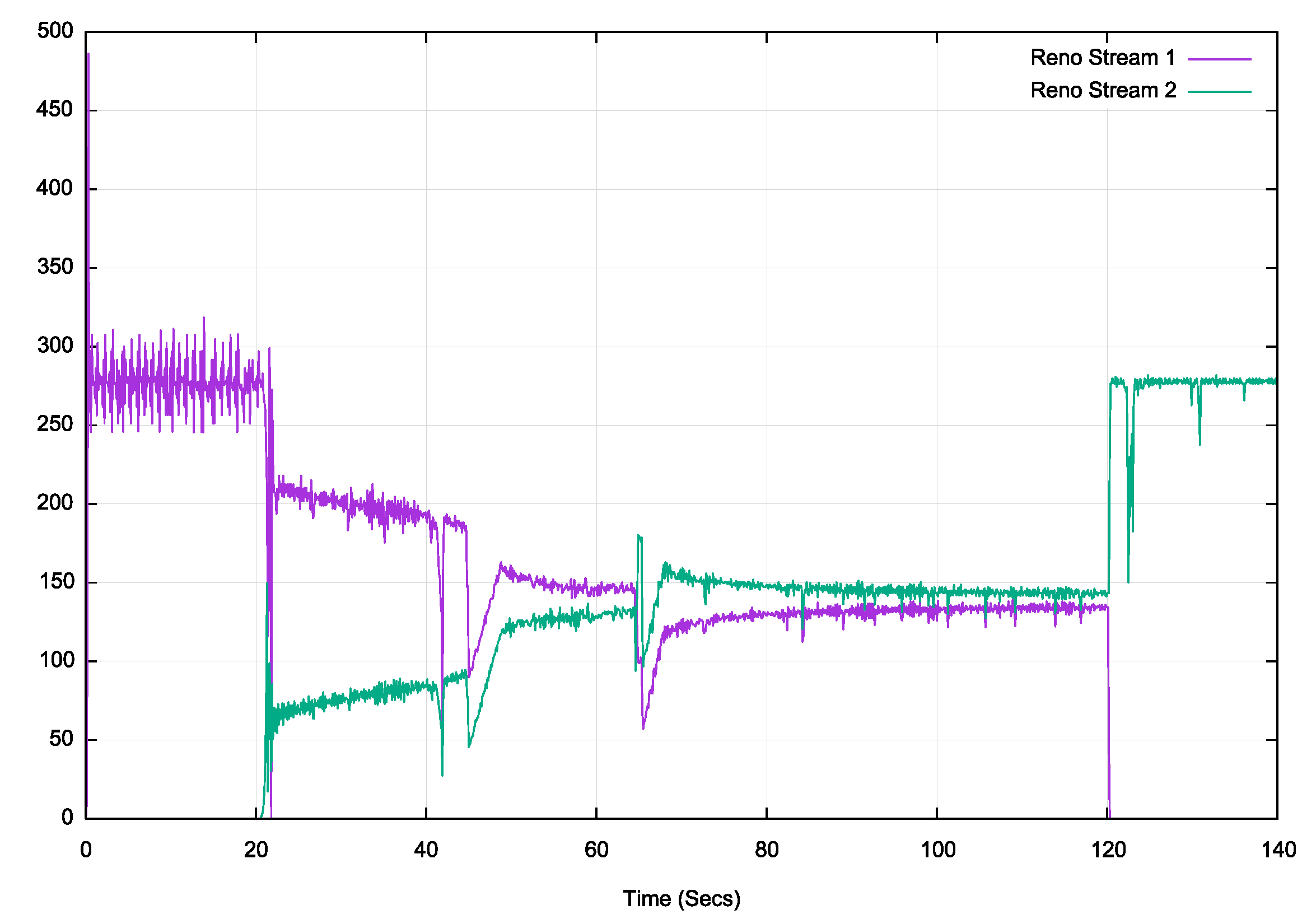
Figure 5 – Reno download over fibre
It’s clear that Reno is able to find the path capacity very quickly and has stabilised on the link capacity within 0.4 of a second, or 40 RTT intervals. When the second Reno stream starts, the initial division of the path capacity is at a ratio of 3:1 between the two streams. It takes a further 80 seconds, or some 400 RTT intervals for the two sessions to stabilize on a roughly equal division of the available path capacity. When the first session stops, the second session quickly fills the available path capacity. This is not a conventional Reno inflation of the sending rate by 1 MSS per RTT. The rapid change in the sending rate in stream 2 points to the use of a Linux kernel structure that holds the current estimate path capacity per destination address, and when one stream finishes, then the other stream is rapidly inflated to occupy the entire path capacity.
Figure 6 shows the same 2 stream measurement, using the Cubic flow control protocol.
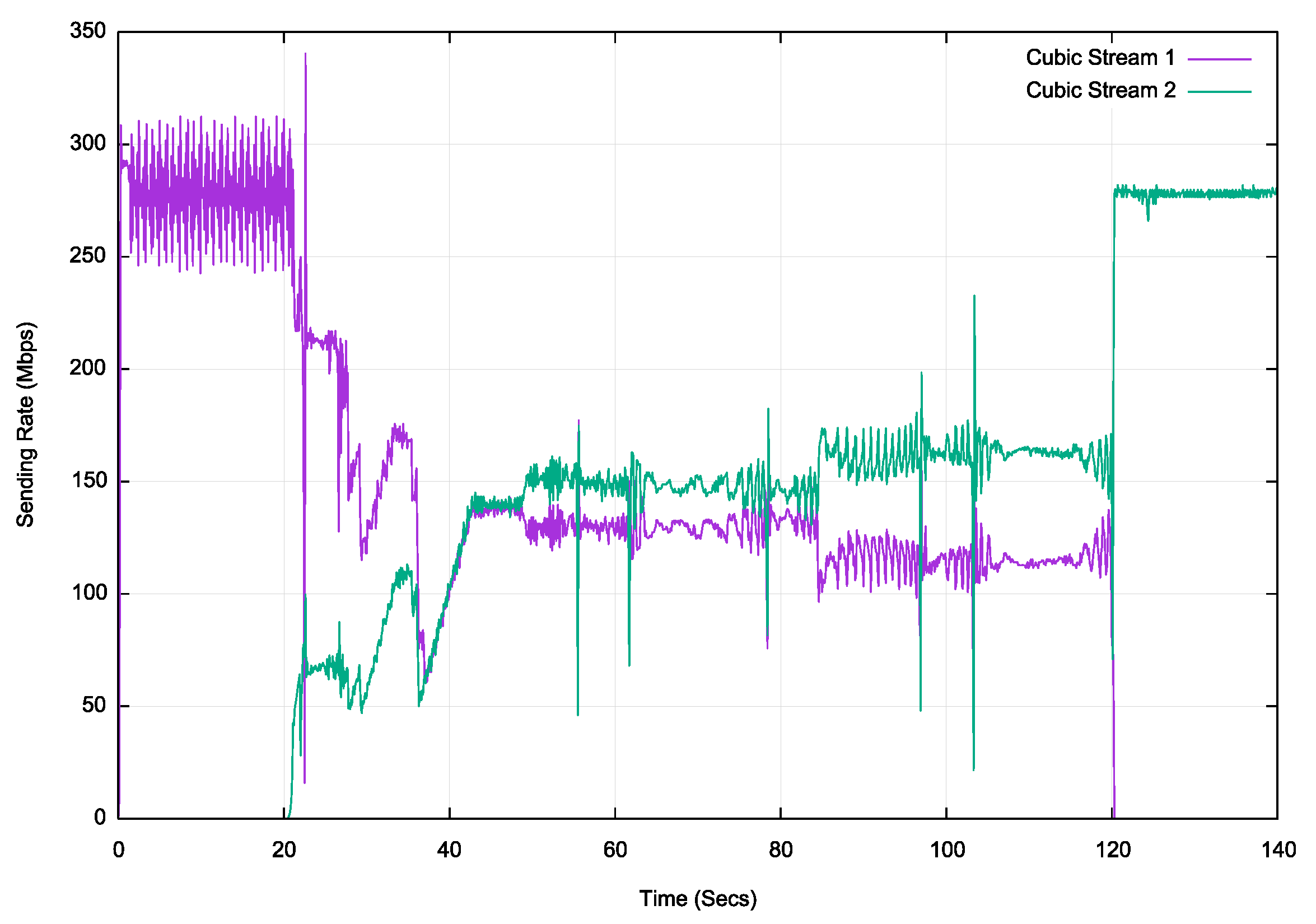
Figure 6 – Cubic download over fibre
The Cubic test behaves in a number of different modes here. The initial start of stream 1 shows a high level of variation in the sending rate, varying the sending rate by 75Mbps over successive 100ms intervals (5 RTT intervals). The last 20 seconds of stream 2 shows a far more stable sending rate. This is quite similar to the behaviour of Reno. Unlike Reno, the two Cubic streams cannot sustain an equal sharing of the link capacity over an extended period of time.
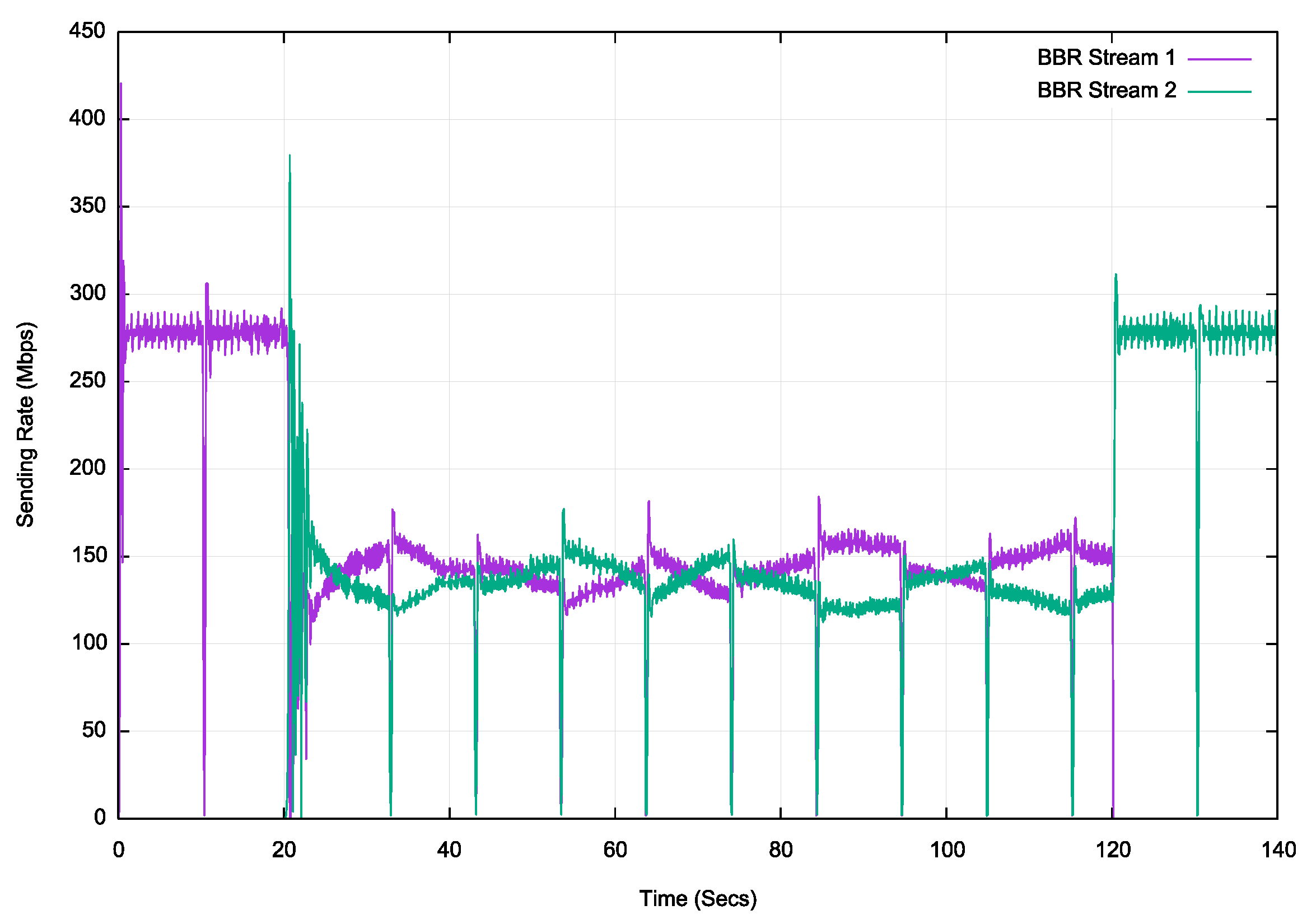
Figure 7 – BBR download over fibre
BBR appears to be a more stable protocol in this scenario. Once BBR establishes the link capacity it maintains it with very small high frequency variation. When the second stream opens, it takes 2.5 seconds (approximately 125 RTT intervals) for the two streams to equalize and maintain this state.
Geo-Stationary Satellite Service
Now let’s look at the other extreme on terms of end-to-end delay, namely a geo-stationary satellite service.
As already noted, the satellite is at an altitude of 35,786km, so the minimum signal propagation distance for a round trip using this satellite service is 143,144 km, or some 477ms. The measured round-trip time is somewhat higher when using a server located in Brisbane, Australia, and, as shown in Figure 8, the measured RTT is some 660ms. The instability of the ping measurements would tend to indicate the build up of internal queues within the terrestrial feeder network. This is an IPv4 only service, so there is only a single ping trace. This was a small ping test (500 samples), but there was no packet loss.
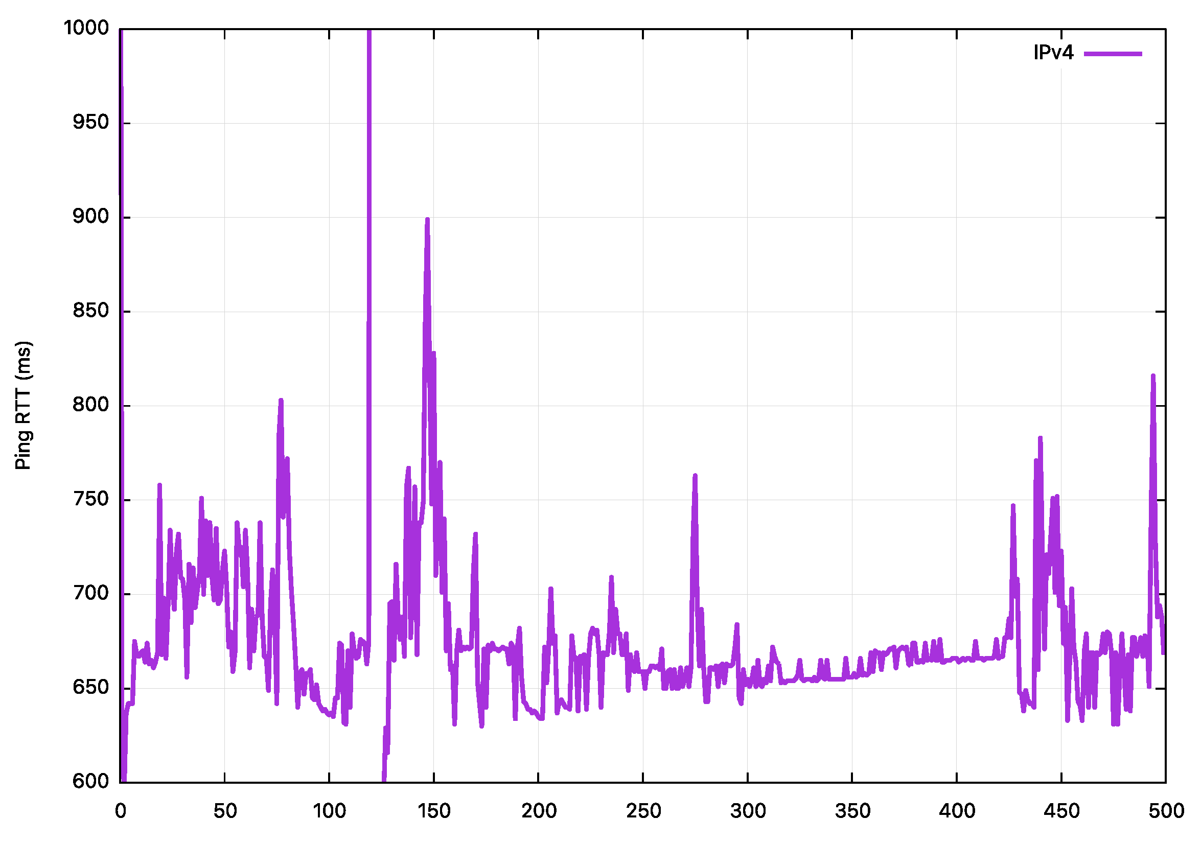
Figure 8 – Ping measurements of the RTT for a GeoStationary Satellite service
These are not ideal conditions for efficient TCP service. The long RTT means that the TCP sender takes up to half a second to respond to changes in the characteristics of the forwarding path, and the high levels of jitter means that the sender’s smoothed RTT estimate will also be off by up to 100ms.
Let’s move on to a downlink test of a 45 Mbps service provided through a geostationary satellite. As with fibre, we will use a 2-stream test, starting one stream 40 seconds earlier than the second. The first of the traces of stream throughput is using the Reno flow control protocol.
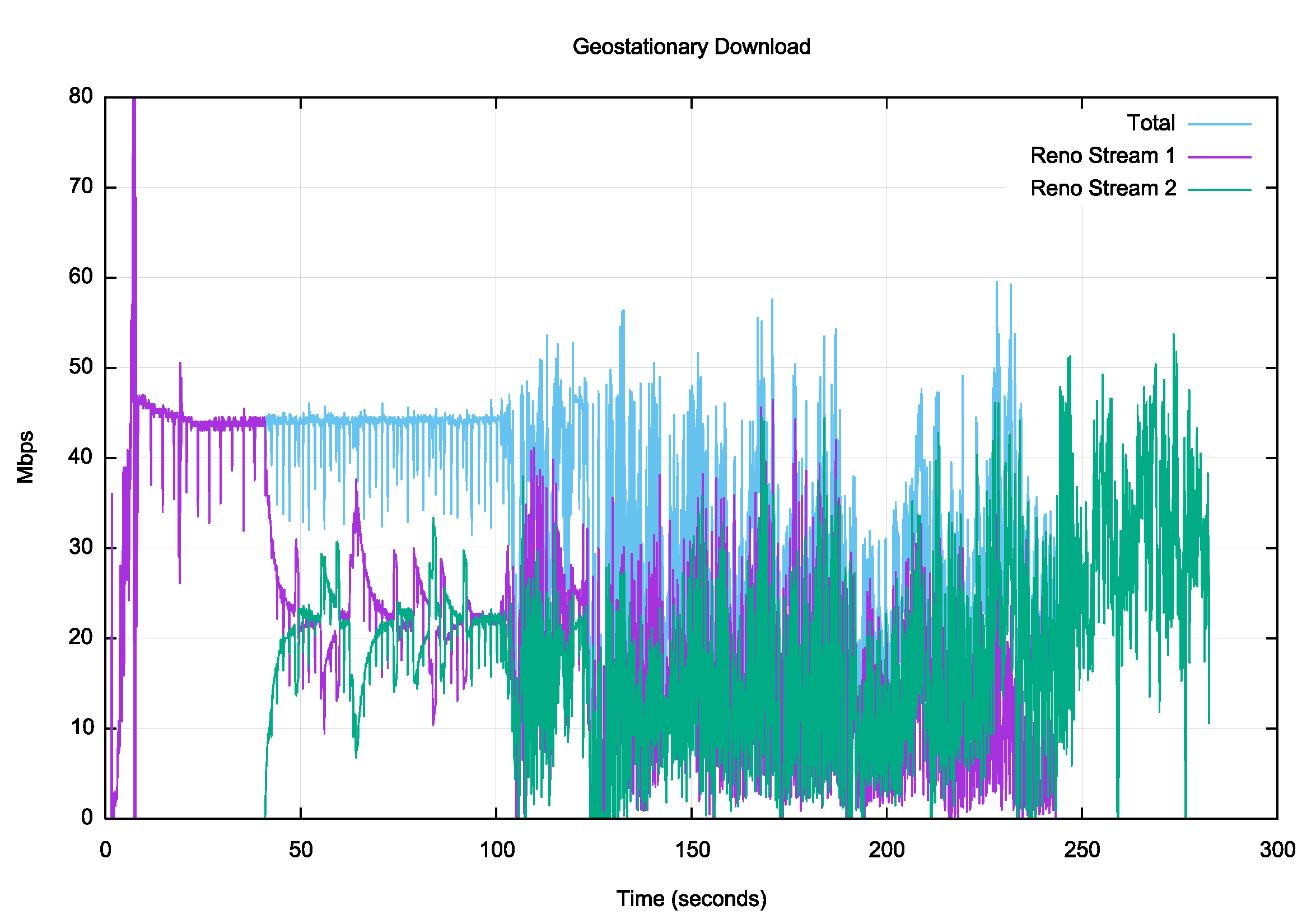
Figure 9 – Reno download over a geostationary satellite service
It appears that this particular satellite service uses large internal queues. These two streams are able to share the available bandwidth for 60 seconds in a relatively stable manner. However, when this situation was disrupted at the 105 second point (possibly due to cross-pressure from some external sessions) both Reno sessions became unstable. The result was that total link efficiency dropped by more than 50%. When the first stream stopped at the 240 second point the second stream was still unable to reestablish a stable flow profile. The combination of high latency, large queues and capacity contention across multiple users creates extended periods of high instability in this service, and this flow control algorithm cannot reestablish stability.
Can the Cubic algorithm fare any better under these conditions? Figure 10 shows the same experiment using Cubic.
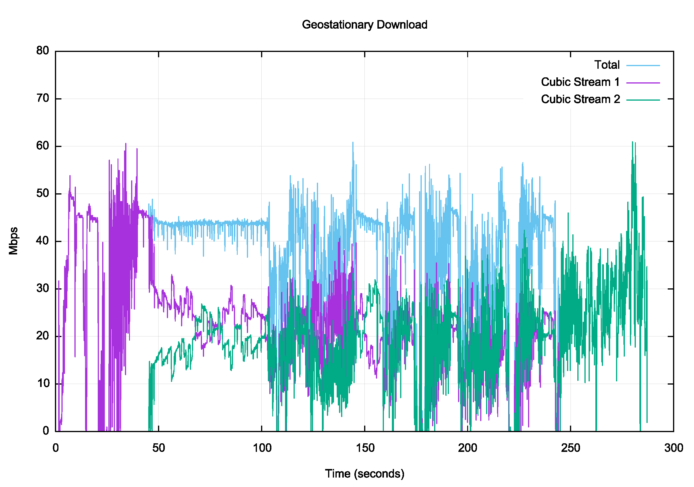
Figure 10 – Cubic download over a geostationary satellite service
There are the same patterns of disruption in the service, and the same unstable response from the Cubic streams as was seen in Reno in Figure 9. Cubic appears to extract a higher level of efficiency of use of the service when the streams are unstable.
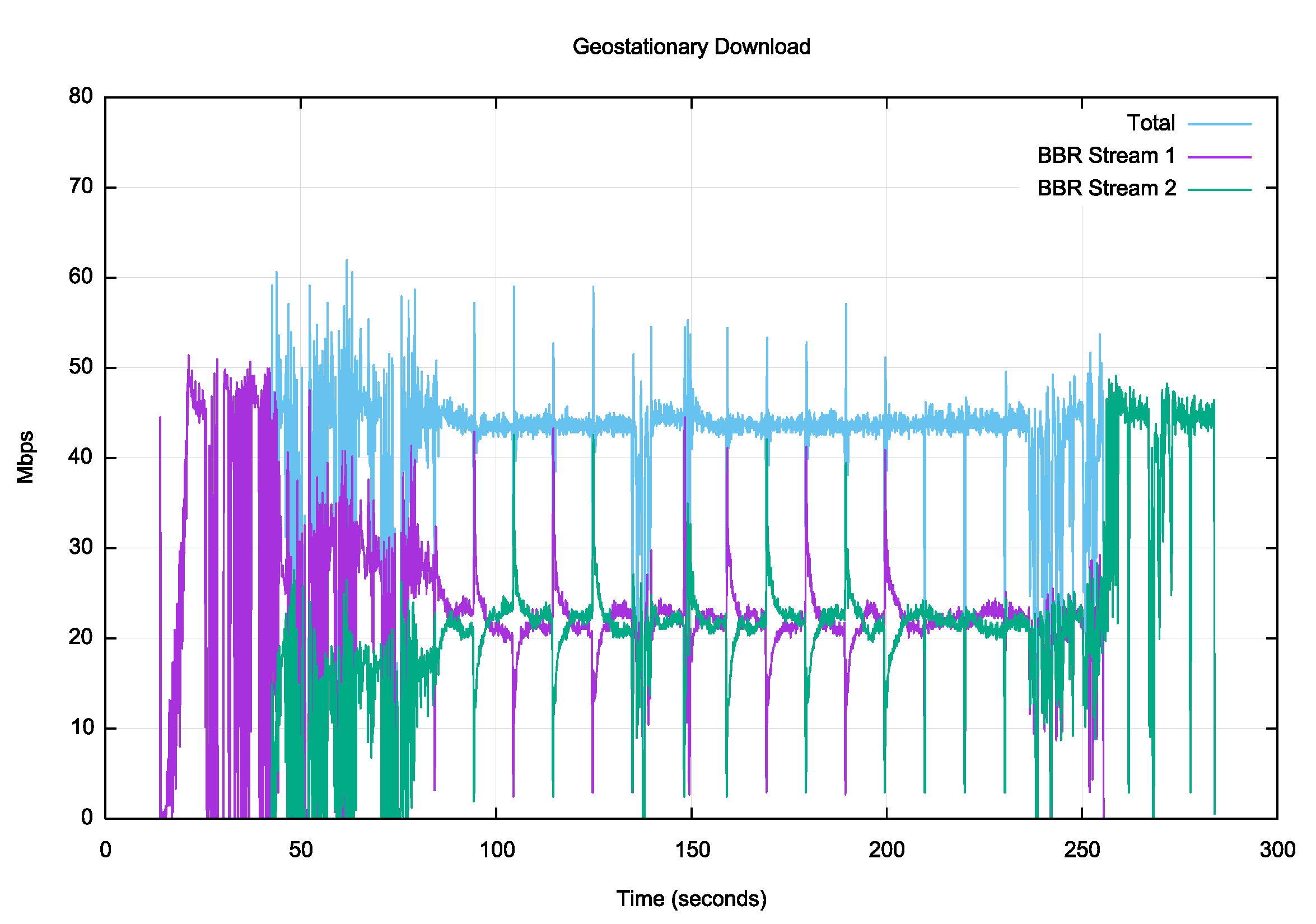
Figure 11 – BBR download over a geostationary satellite service
BBR appears to be far more capable of pushing back into the network to sustain a stable flow rate (Figure 11). This algorithm attempts to maintain a constant sending rate into the network for sequences of 6 successive RTT intervals, which is reflected in the imposition of a stable sending rate for most of the time. The two streams rapidly equilibrate and share the available path capacity, and they combine to sustain a highly efficient use of the circuit.
Any path with such a high RTT is a challenge to use efficiently, and if you add jitter, large buffers, and the periodic build-up of standing queues, then the outcome is quite hostile to efficient TCP flow control algorithms. In this limited experiment it appears that BBR clearly produces a better outcome under these quite challenging conditions.
LEO Satellite Service
Let’s now look at the service offered by Starlink. A ping test with 2,000 samples shows an interesting result:
2000 packets transmitted, 1991 received, 0.45% packet loss, time 2009903ms
rtt min/avg/max/mdev = 37.284/60.560/214.301/13.549 ms
Firstly, there is some packet loss present, with 9 ping packets lost out of the 2,000 that were sent. It is unclear if this is due to rain fade or satellite tracking handover or a combination of the two. Secondly, there is a high rate of variation of the RTT measured by this test. The minimum RTT was 37ms, while the average is 60.5ms and the mean standard variation is 13.5ms. The plot of the ping delays is shown in Figure 12.
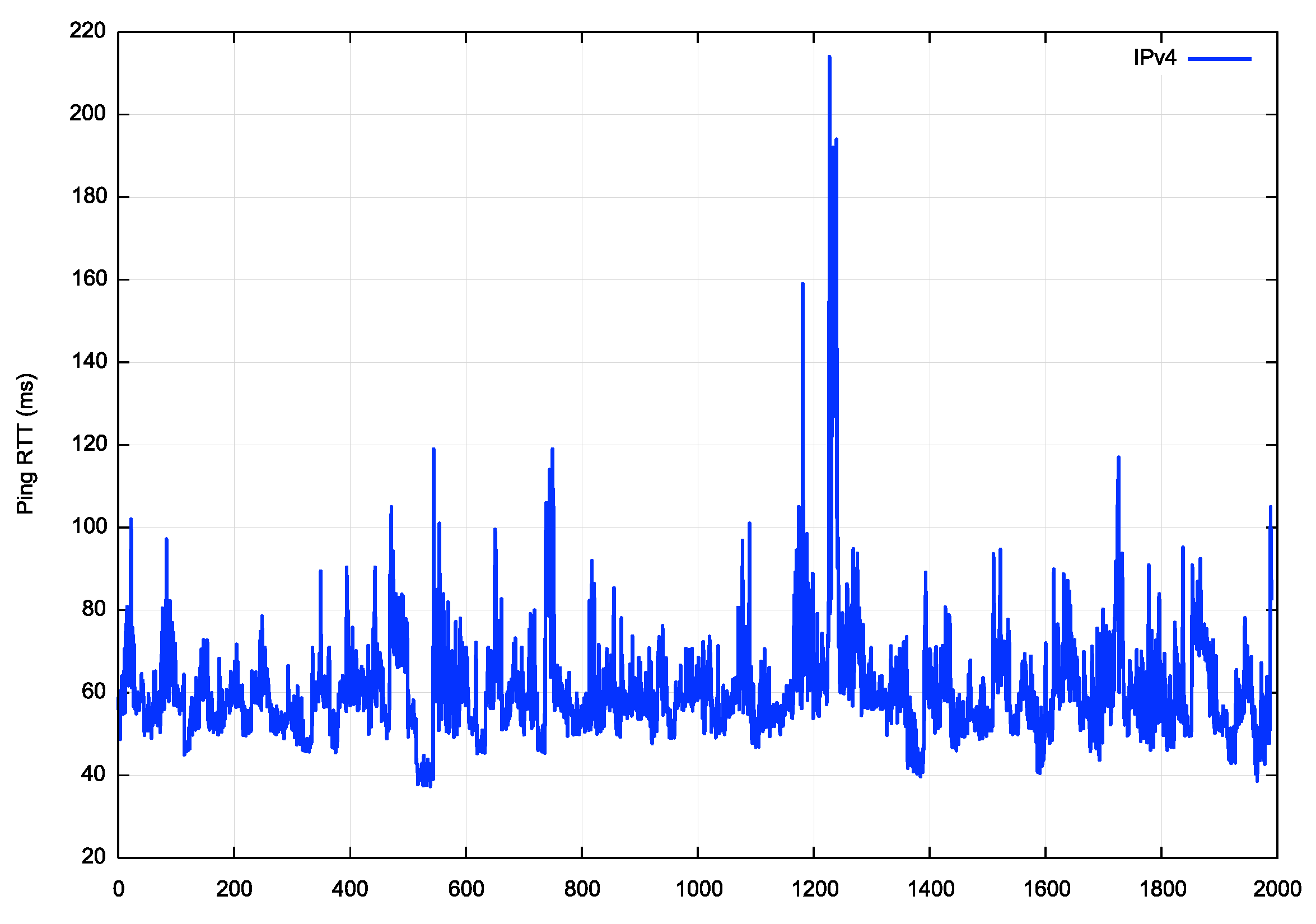
Figure 12 – Ping measurements of the RTT for the Starlink LEO Satellite service
The transmission delays for this service include some 12ms of terrestrial network, and the remainder is associated with the satellite link. The distance between the satellite and a visible earth station varies between 550km when the satellite is directly overhead and 2,704km when the satellite is on the horizon. This correlates to a one-way signal propagation time of between 1.8 and 9ms, or a potential variation in RTT times of between 7.3 and 36ms. There are also encryption delays and presumably codec delays, so the overall delivered RTT performance was observed to be an average 60ms for this service with a variation of +/- 13ms, which matches the geometry of the LEO constellation It is not clear whether the isolated RTT measurements of in excess of 100ms are due to crosstalk or satellite tracking handover.
Let’s now turn to the download performance of this Starlink service.
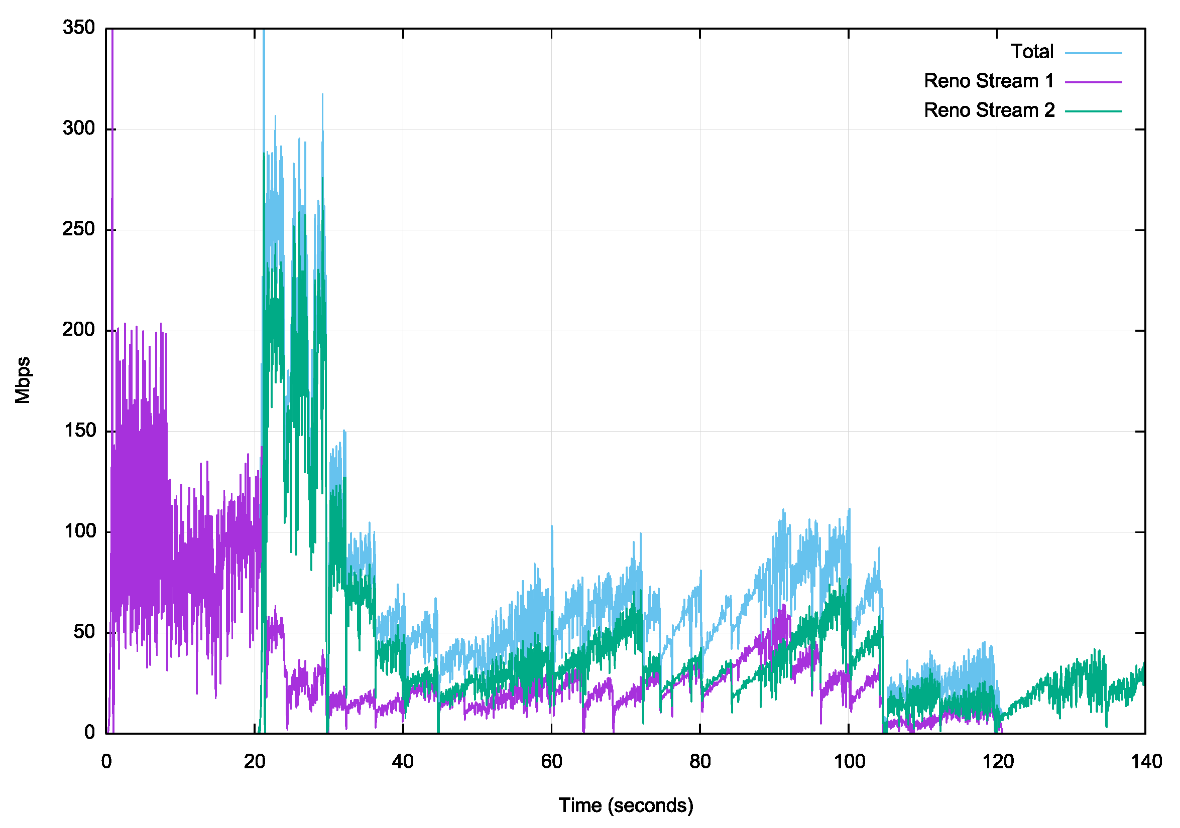
Figure 13 – Reno download over Starlink LEO service
The constantly changing RTT of this service appears to have thrown the Linux settings that allow the sender to latch onto a path capacity to a destination address and maintain it. The signature Reno linear inflation of the sending rate and the periodic rate halving is now clearly visible. The increased packet loss probability of this Starlink service limits the ability of Reno to open its cwnd, and the overall path capacity is not sustainable over 100Mbps (Figure 13).
Cubic fares no better here. The classic Cubic pattern of window inflation and rate halving can be seen from second 20 to second 55. The constantly varying RTT appears to prevent the Linux drivers from “latching” onto a sustainable path capacity rate, and the sporadic packet loss events prevent the Cubic streams from opening up the sending window.
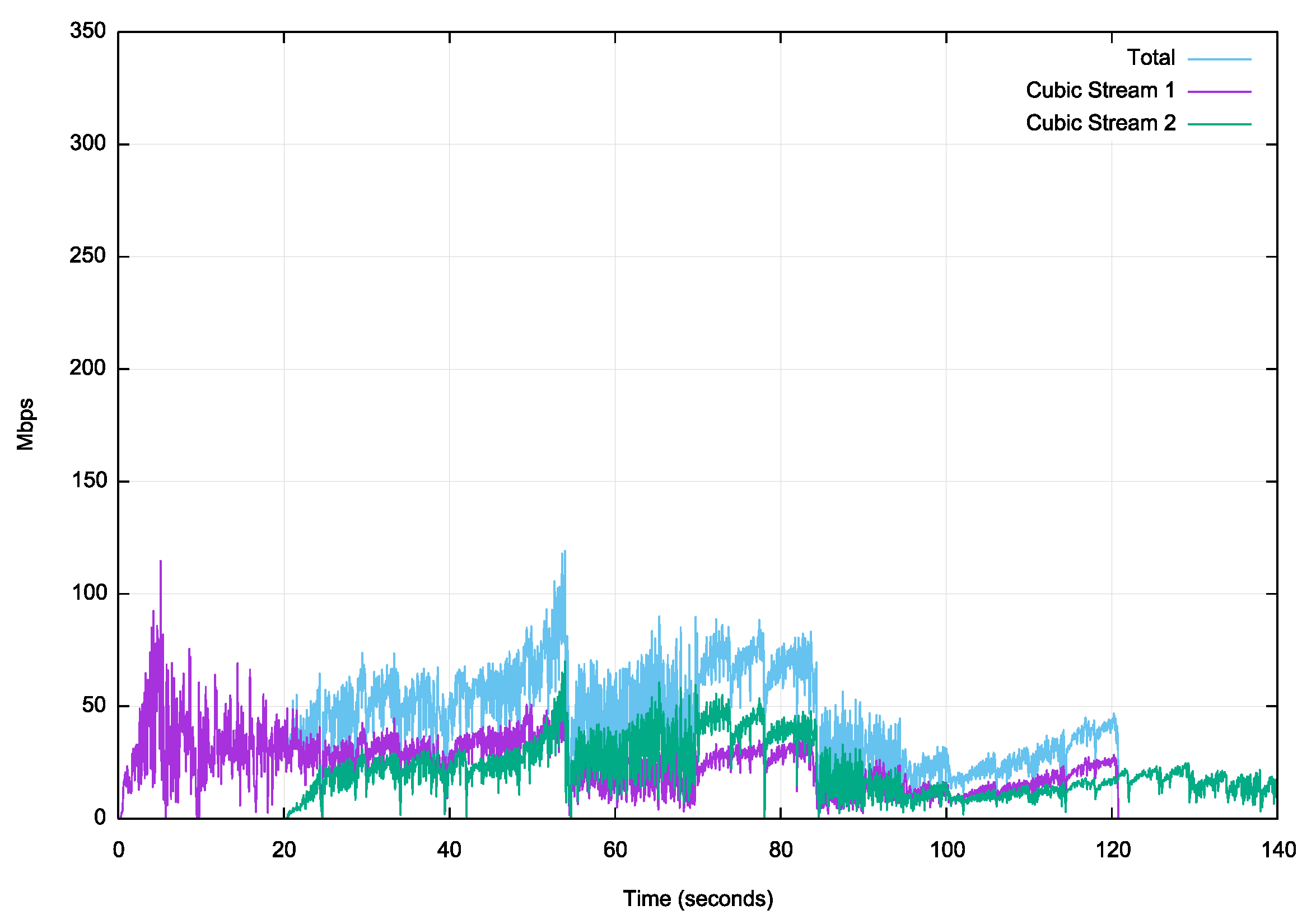
Figure 14 – Cubic download over Starlink LEO service
It takes approximately 20 seconds for the two streams to reach the notional path capacity of 90Mbps, and the incidence of packet loss causes the collapse of the sending window, which is not subsequently recovered.
BBR appears to be far more successful here. A single BBR session appears to be able to drive the network path at a capacity of between 150Mbps – 200Mbps. When there are 2 active BBR sessions, then BBR finds it challenging to stabilize at any particular sending rate, and it is constantly making adjustments. While the sending rate is not stable, BBR achieves considerably greater overall throughput than either Reno or Cubic under these conditions.
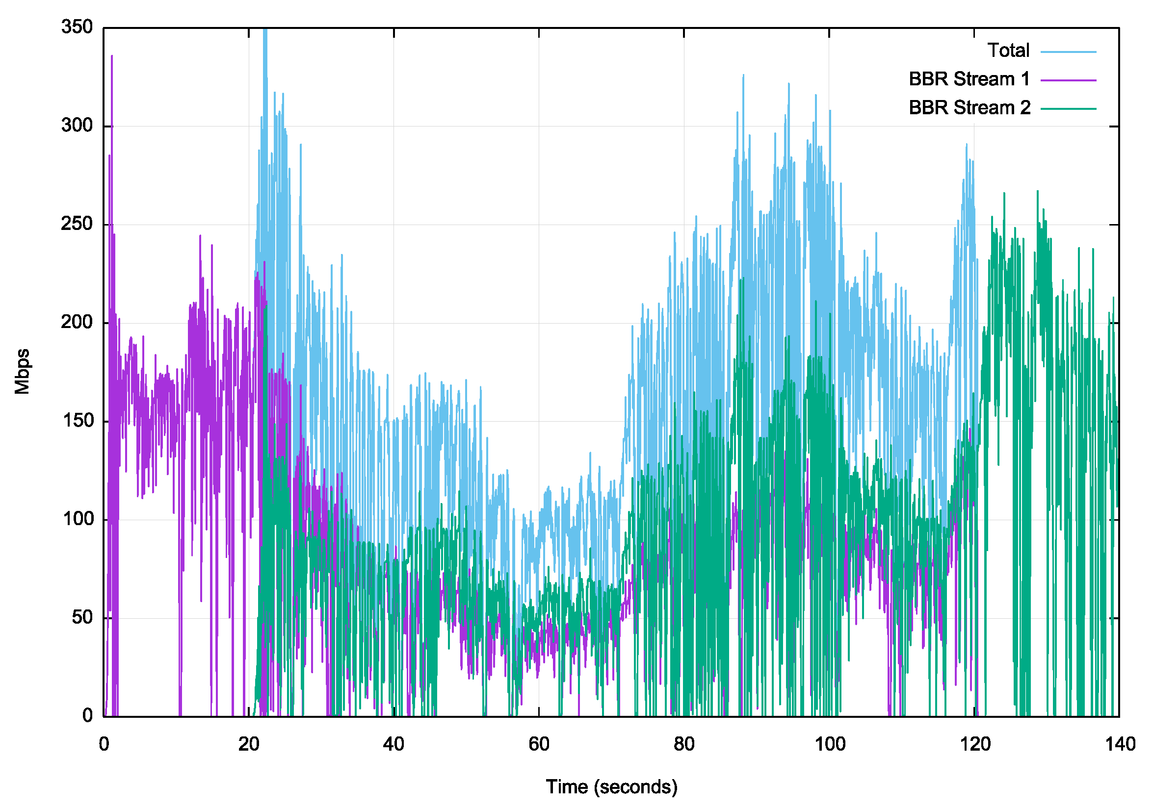
Figure 15 – BBR download over Starlink LEO service
Conclusions
In many respects this has been a surprising investigation.
The Linux implementation of TCP has some unanticipated behaviours. There appears to be an overlay element in the kernel that assumes control of the TCP session if it believes that the path capacity to the destination and its RTT are stable. The Linux kernel’s route cache has undergone some changes over the various Linux versions, but the system still behaves in a way that attempts to associate destinations with a cached path capacity value and “latch” the TCP sending rate to this capacity value. In both the fibre and geostationary service profiles we cannot directly observe the “sawtooth” periodic sending behaviour of AIMD control algorithms, nor the polynomial curves associated with Cubic. In its place we seen the sender rapidly lock onto the path capacity and maintaining this constant sending rate. This is an extremely effective outcome for the user, in that the TCP sender is able to rapidly drive a network path at capacity and sustain this sending rate over extended periods of time.
It’s also evident that there are network paths whose characteristics disable this managed performance TCP behaviour, as this steady state sending behaviour is not evident in the Starlink test, where we see the result of conventional TCP control algorithms controlling the sending rate. It is unclear to me what characteristics and thresholds control this TCP override. Up to date documentation of this aspect of Linux TCP behaviour is not readily available.
This host TCP behaviour is further compounded by the behaviour of modern network interfaces which are performing offloading of TCP segmentation and checksums, which is most relevant for high speed paths, where a significant proportion of the per-packet processing loads are effectively shunted over to the network interface processor.
Where there is a stable network path, then Linux is extremely good in driving the network to the point of maximal efficiency. For low delay high capacity paths, such as terrestrial fibre, it does not make much difference whether Reno, Cubic or BBR is used as the TCP flow control protocol. Linux will operate the network path at maximal efficiency.
The BBR protocol operates surprisingly well over geostationary satellite services. These high latency services present many challenges for feedback-controlled flow systems because of the significant lag in providing feedback to the server, but BBR appears to manage this situation far more efficiently than the other two loss-based control algorithms. However, none of these TCP protocols can compensate for the high end-to-end path latency, so these geostationary satellite services are ineffective in providing highly responsive services. The lag between command and response cannot be avoided. If the application is based on high volume data transfer, then it is possible for a combination of a Linux host and the BBR TCP algorithm to drive these services at maximal efficiency.
The Starlink LEO service has some unexpected characteristics. The packet loss rate is higher than expected, and this may be an outcome of the combination of using phase array antennae that are tracking satellites that are moving through the sky at a relative speed of 1 degree of elevation every 15 seconds, together with the need to perform satellite handover at regular intervals. The client dish of not a very high power transmitter, so there is also the issue of rain fade that will degrade the service during showers.
The RTT variance is this service is also higher than expected. However, even with a 60ms RTT, the responsiveness of this service is at a level that any geostationary service simply cannot emulate.
When used with Linux endpoints, the choice of TCP flow control protocol appears to be critical for a Starlink service. Both Reno and Cubic were observe to collapse, while BBR was able to extract highly efficient performance over this Starlink service.
TCP is at its most efficient over low latency highly stable infrastructure, so these satellite services are poor substitutes for a terrestrial service. If responsiveness is important, which is often the case for voice and video applications, then Starlink is the logical choice, due to a RTT latency which is a fraction of the RTT of any geostationary service. However, it appears that the choice of which TCP control protocol to use is a critical factor here.
For closed environments where there is control of both the sender and receiver it is possible to tune TCP to make optimal use of these satellite services, and in these experiments the use of BBR appears to be a clear preference. However, in the public Internet there is no such tight control over every content source, and a server has no a priori knowledge of the characteristics of the path to reach the client. For many years the conventional wisdom has been to rely on ample provisioning of internal queues within the network in an attempt to minimise packet loss events and generalise the network behaviour to adequately respond to most forms of traffic management over diverse paths. Recent research is now pointing in a different direction, where the combination of small network queues and delay sensitive end-to-end control algorithms can provide extremely efficient service outcomes. However, mapping this requirement for highly stable underlying path propagation delays into the LEO environment is going to pose some challenges for the LEO folk. Even so, in networking, delay is almost everything, and many other issues become far more tractable when the underlying end-to-end latency is short. For that reason, LEO systems will continue to be a very attractive solution to many rural and remote connectivity requirements.
Acknowledgements
This measurement has proved to be far more challenging than was originally envisaged. Siting a Linux server in an unattended remote location is always going to be a challenge and I am indebted to APNIC’s Paul Wilson and George Michaelson for setting up and installing the measurement system to perform these tests.
While setting up runs of iperf3 and performing a packet capture of the actual file transfers was relatively straightforward, the task of relating the observed TCP behaviour to the documented Linux behaviours has been very frustrating at times. Thanks to Joao Damas of APNIC for assisting me in working through what folk optimistically label as “Linux documentation” and discovering the tcp_probe kernel diagnostic!